EXPERIMENTS: INTRODUCTION-HYPOTHESIS TEST-SAMPLE SIZE (DATA SCIENCE 2018)
Toni Monleon-Getino (Section of Statistics, Faculty of Biology. Group of Research BIOST3, GRBIO)
16 de OCTUBRE de 2017
INTRODUCTION
The aim of this tutorial is to review the concepts of a first course in biostatistics within the university postdegree and introduce the analysis of the experiments.
- See a good introduction at: A First Course in Design and Analysis of Experiments
- Theory introduction at: Probabilitat i estad?stica per a ci?ncies MONLEON T, RODRIGUEZ C. Probabilitat i estadistica per a ciencies I. PPU. BARCELONA. 2015.
# A first example of data (weight in kg)

x <- rnorm(25,34,5)
x
## [1] 32.97336 38.14072 25.50829 27.24743 31.47995 31.97935 38.17831
## [8] 32.66663 31.00241 28.04502 38.64170 32.60191 37.72771 34.03477
## [15] 35.21323 35.11539 29.78396 30.19848 30.62769 34.07139 29.51789
## [22] 36.17243 30.81579 28.20188 35.34892summary(x)## Min. 1st Qu. Median Mean 3rd Qu. Max.
## 25.51 30.20 32.60 32.61 35.21 38.64hist(x)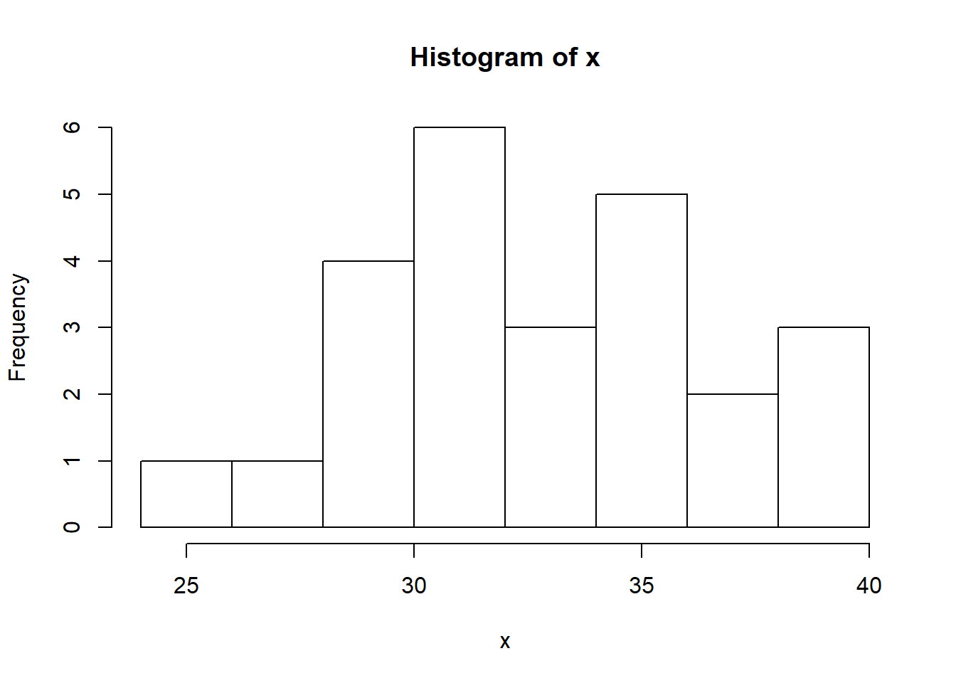
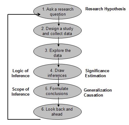
The scientific method
A hypothesis is a proposed explanation for a phenomenon. For a hypothesis to be a scientific hypothesis, the scientific method requires that one can test it. Scientists generally base scientific hypotheses on previous observations that cannot satisfactorily be explained with the available scientific theories.
WHy experiments?
An experiment is characterized by the treatments and experimental units to be used, the way treatments are assigned to units, and the responses that are measured.
Researchers use experiments to answer questions. Typical questions might Experiments answer questions be:
- Is a drug a safe, effective cure for a disease?
- This could be a test of how AZT affects the progress of AIDS
- Which combination of protein and carbohydrate sources provides the best nutrition for growing lambs?
- How will long-distance telephone usage change if our company offers a different rate structure to our customers?
- Which combination of protein and carbohydrate sources provides the best nutrition for growing lambs?
- Will an ice cream manufactured with a new kind of stabilizer be as palatable as our current ice cream?
- Does short-term incarceration of spouse abusers deter future assaults?
- Under what conditions should I operate my chemical refinery,given this month’s grade of raw material?

Experiments help us answer questions
Experiments help us answer questions, but there are also non experimental techniques. What is so special about experiments?
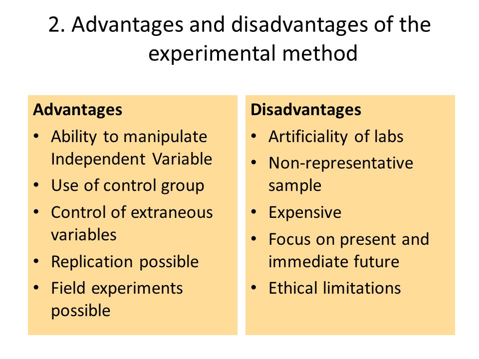
Consider use experiments for its Advantages:
- 1.Experiments allow us to set up a direct comparison between the treatments of interest.
- 2.We can design experiments to minimize any bias in the comparison.
- 3.We can design experiments so that the error in the comparison is small.
- 4.Most important, we are in control of experiments, and having that control allows us to make stronger inferences about the nature of differences that we see in the experiment. Specifically, we may make inferences about causation
But not all are adventages:
We can distinguish between observational and experimental studies See at:
The Statistical method
Statistics is the science of learning from data, and of measuring, controlling, and communicating uncertainty; and it thereby provides the navigation essential for controlling the course of scientific and societal advances (Davidian, M. and Louis, T. A., 10.1126/science.1218685).Statisticians apply statistical thinking and methods to a wide variety of scientific, social, and business endeavors in such areas as astronomy, biology, education, economics, engineering, genetics, marketing, medicine, psychology, public health, sports, among many. “The best thing about being a statistician is that you get to play in everyone else’s backyard.” (John Tukey, Bell Labs, Princeton University)
Many scientific, medical, economic, social, political, and military decisions cannot be made without statistical techniques, such as the design of experiments to gain federal approval of a newly manufactured drug.
HYPOTHESIS TEST
How the statistical hypothesis test work?
In many cases, the researcher has an a priori belief, possibly based on his previous experience with the phenomenon being studied on the numerical values of the parameters of this process. In this case, the researcher is interested in estimating the numerical values of these parameters are unknown, but may also want to compare several hypotheses about the probability distribution of the population that generated the sample available.Generally assumptions relate to whether the sample information is consistent with his belief a priori on the parameter values, which formed the so-called problems of a sample.
Sometimes the researcher has two samples, and questioned whether the information provided is both consistent with the possibility that come from the same population, against the alternative that comes from different populations, these problems called two samples.
Then a hypothesis is a statement about the statistical characteristics of a process, which can be considered a hypothesis and conjecture. For example, if a scientist observes energy at a certain metabolic process for several hours, you know the average consumption of the hours noted. With the help of inference, can advance a step further and speculate if the average consumption of all reactions observed is a certain value or another. The scientific process is then tested their hypothesis against an alternative hypothesis.
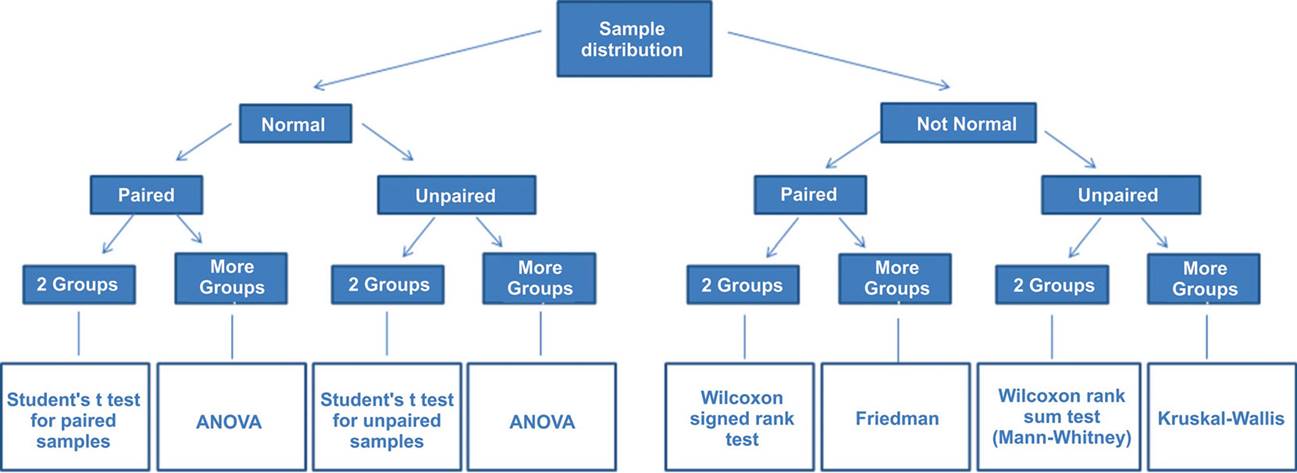
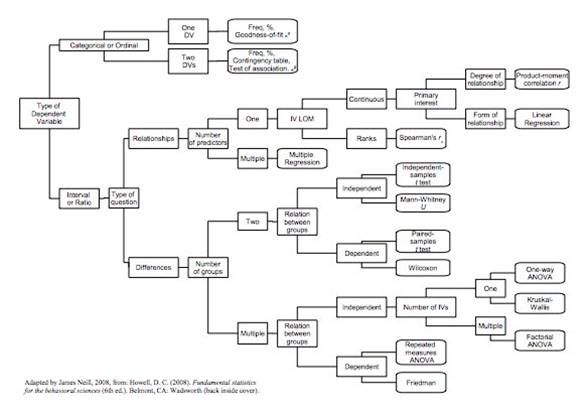
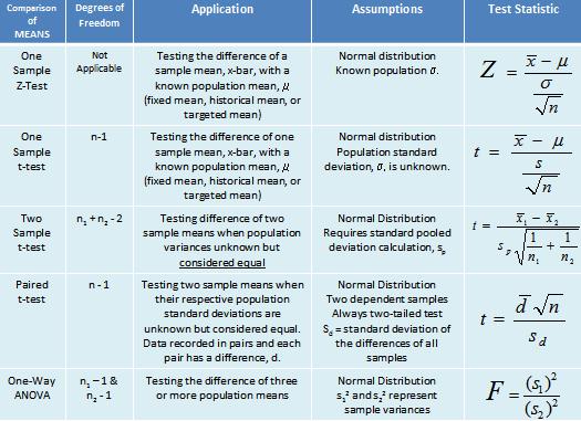
The steps in the hypothesis testing procedure are:
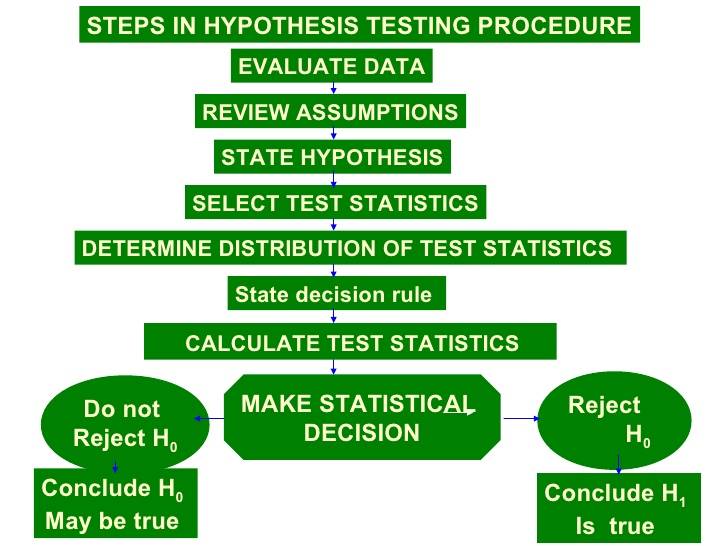
We can find algorithms to help us in the statistical method used. Obviously all it based on the theory of probability and statistics.
Some of the algorithms can be found below in the following figures.

And anothers depending on the the characteristics of the sample and the types of probability distributions:
See information about hyphotesys test at this link:
More information at:
Probabilitat i estadistica per a ciencies MONLEON T, RODRIGUEZ C. Probabilitat i estadistica per a ciencies I. PPU. BARCELONA. 2015.
Some useful probability distributions
Normal (Gaussian) distribution:
In probability theory, the normal (or Gaussian) distribution is a very common continuous probability distribution. Normal distributions are important in statistics and are often used in the natural and social sciences to represent real-valued random variables whose distributions are not known.[1][2]
See function at https://en.wikipedia.org/wiki/Normal_distribution
The normal distribution is useful because of the central limit theorem. In its most general form, under some conditions (which include finite variance), it states that averages of random variables independently drawn from independent distributions converge in distribution to the normal, that is, become normally distributed when the number of random variables is sufficiently large. Physical quantities that are expected to be the sum of many independent processes (such as measurement errors) often have distributions that are nearly normal.[3] Moreover, many results and methods (such as propagation of uncertainty and least squares parameter fitting) can be derived analytically in explicit form when the relevant variables are normally distributed.
The normal distribution is sometimes informally called the bell curve. However, many other distributions are bell-shaped (such as the Cauchy, Student’s t, and logistic distributions). The terms Gaussian function and Gaussian bell curve are also ambiguous because they sometimes refer to multiples of the normal distribution that cannot be directly interpreted in terms of probabilities.
EXAMPLE: We can see an example of use of Normal distribution: Children’s IQ scores are normally distributed with a mean of 100 and a standard deviation of 15. What proportion of children are expected to have an IQ between 80 and 120?
mean=100; sd=15
lb=80; ub=120

x <- seq(-4,4,length=100)*sd + mean
hx <- dnorm(x,mean,sd)

plot(x, hx, type="n", xlab="IQ Values", ylab="",
  main="Normal Distribution", axes=FALSE)

i <- x >= lb & x <= ub
lines(x, hx)
polygon(c(lb,x[i],ub), c(0,hx[i],0), col="red")

area <- pnorm(ub, mean, sd) - pnorm(lb, mean, sd)
result <- paste("P(",lb,"< IQ <",ub,") =",
   signif(area, digits=3))
mtext(result,3)
axis(1, at=seq(40, 160, 20), pos=0) 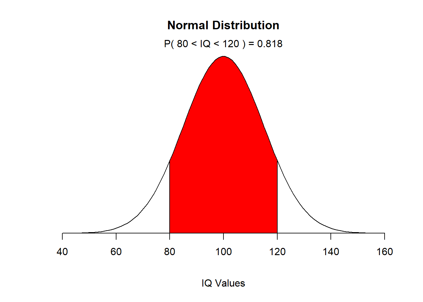
T Student distribution
In probability and statistics, Student’s t-distribution (or simply the t-distribution) is any member of a family of continuous probability distributions that arises when estimating the mean of a normally distributed population in situations where the sample size is small and population standard deviation is unknown. It was developed by William Sealy Gosset under the pseudonym Student. Whereas a normal distribution describes a full population, t-distributions describe samples drawn from a full population; accordingly, the t-distribution for each sample size is different, and the larger the sample, the more the distribution resembles a normal distribution.
See information T Student at this link:
# An example of a T Student distribution and its comparison with a normal

# Display the Student's T distributions with various degrees of freedom and compare to the normal distribution

x <- seq(-4, 4, length=100)
hx <- dnorm(x) #simulate a normal distribution

degf <- c(1, 3, 8, 30)
colors <- c('red', 'blue', 'darkgreen', 'gold', 'black')
labels <- c('df=1', 'df=3', 'df=8', 'df=30', 'normal')

plot(x, hx, type='l', lty=2, xlab='x value',
  ylab='Density', main='Comparison of t Distributions')

for (i in 1:4){
  lines(x, dt(x,degf[i]), lwd=2, col=colors[i])
}

legend('topright', inset=.05, title='Distributions',
  labels, lwd=2, lty=c(1, 1, 1, 1, 2), col=colors)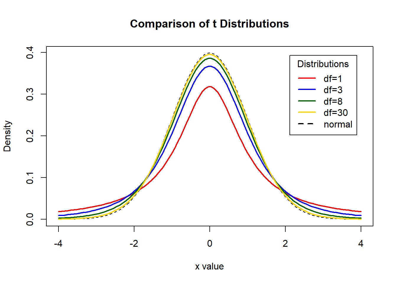
Chi-Squared distribution
See information Chi square distribution at this link:
In probability theory and statistics, the chi-squared distribution (also chi-square or ji-distribution) with k degrees of freedom is the distribution of a sum of the squares of k independent standard normal random variables. It is a special case of the gamma distribution and is one of the most widely used probability distributions in inferential statistics, e.g., in hypothesis testing or in construction of confidence intervals.[2][3][4][5] When it is being distinguished from the more general noncentral chi-squared distribution, this distribution is sometimes called the central chi-squared distribution.
The chi-squared distribution is used in the common chi-squared tests for goodness of fit of an observed distribution to a theoretical one, the independence of two criteria of classification of qualitative data, and in confidence interval estimation for a population standard deviation of a normal distribution from a sample standard deviation. Many other statistical tests also use this distribution, like Friedman’s analysis of variance by ranks.
# An example of Chi-Squared distribution
x <- rchisq(100, 5)
hist(x, prob=TRUE)
curve( dchisq(x, df=5), col='green', add=TRUE)
curve( dchisq(x, df=10), col='red', add=TRUE )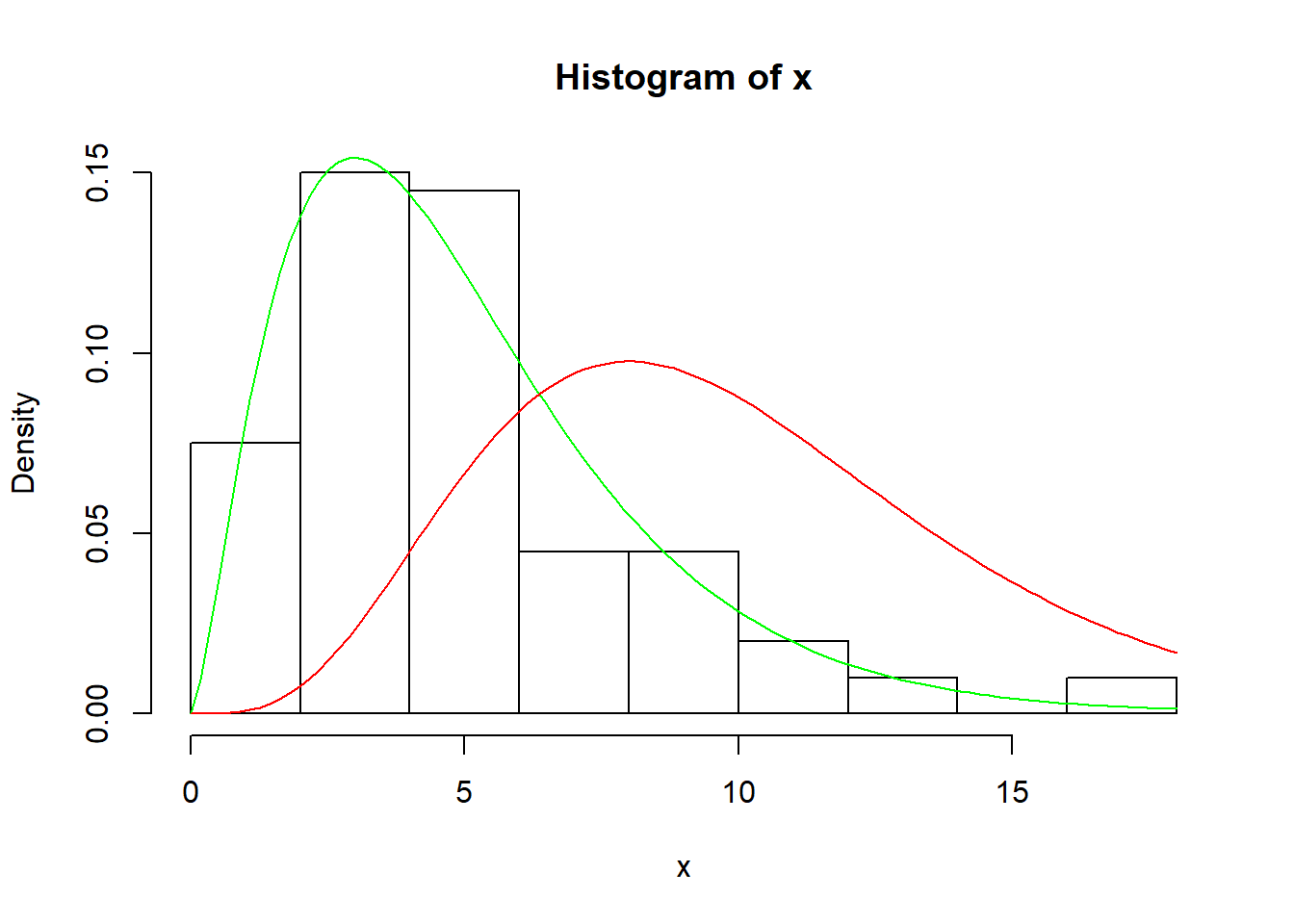
Fisher-Snedecor distribution
Another useful function is the Fisher-Snedecor distribution.
The F-distribution, also known as Snedecor’s F distribution or the Fisher-Snedecor distribution (after Ronald Fisher and George W. Snedecor) is, in probability theory and statistics, a continuous probability distribution.
The F-distribution arises frequently as the null distribution of a test statistic, most notably in the analysis of variance
See information Chi square distribution at this link:
We can draw the density of a Fisher distribution (F-distribution) in the following example:
# An example of Fisher-Snedecor distribution
 par(mar=c(3,3,1,1))
 x <- seq(0,5,len=1000)
 plot(range(x),c(0,2),type="n")
 grid()
 lines(x,df(x,df1=1,df2=1),col="black",lwd=3)
 lines(x,df(x,df1=2,df2=1),col="blue",lwd=3)
 lines(x,df(x,df1=5,df2=2),col="green",lwd=3)
 lines(x,df(x,df1=100,df2=1),col="red",lwd=3)
 lines(x,df(x,df1=100,df2=100),col="grey",lwd=3)
 legend(2,1.5,legend=c("n1=1, n2=1","n1=2, n2=1","n1=5, n2=2","n1=100, n2=1","n1=100, n2=100"),col=c("black","blue","green","red","grey"),lwd=3,bty="n")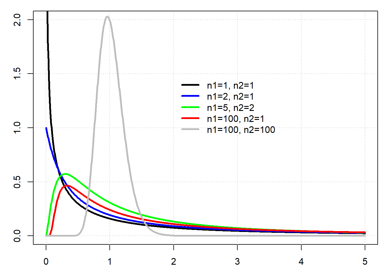
Alfa, Beta (statistical errors)
In statistical hypothesis testing, a type I error is the incorrect rejection of a true null hypothesis (a “false positive”), while a type II error is incorrectly retaining a false null hypothesis (a “false negative”).[1] More simply stated, a type I error is detecting an effect that is not present, while a type II error is failing to detect an effect that is present. The terms “type I error” and “type II error” are often used interchangeably with the general notion of false positives and false negatives in binary classification, such as medical testing, but narrowly speaking refer specifically to statistical hypothesis testing in the Neyman-Pearson framework

EXAMPLE Some athletes use hormones to doping. These hormones can not be used by professional athletes and their use is pursued. The problem is being produced naturally in the human body and the anti-doping agency has difficulty establishing a threshold (via urinalysis) about when an athlete has doped or not. To establish this approach uses a statistical criterion.
Another problem: The cheese can alter the concentration of the natural hormone in the human body.
We represent the probability function for hormone concentration under the null hypothesis (no take cheese) and under the alternative (taking cheese). This probability (model) is normal (gaussian).
Let’ s go to check the distribution of the hormon concentration under two hyphotesis:
Ho: Null hyphotesis (Athletes who do not eat cheese ) mu=7 ng/ml H1: Alternative hyphotesis (Athletes who eat cheese) mu=8.5 ng/ml
 #normal function of probability under null hyphotesis and alternative hyphotesis (mean of 16 atletes)
x<-seq(5,11,length=1000)
y<-dnorm(x,mean=7,sd=(2.4/sqrt(16)))
plot(x,y,type="l",lwd=3,col="blue",cex.axis=2.6,cex.lab=2, xlab = "mg/dL", ylab = "")
y2<-dnorm(x,mean=8.5,sd=(2.4/sqrt(16)))
curve(dnorm(x,mean=8.5,sd=(2.4/sqrt(16))),type="l",lwd=2.6,col="red",add=T)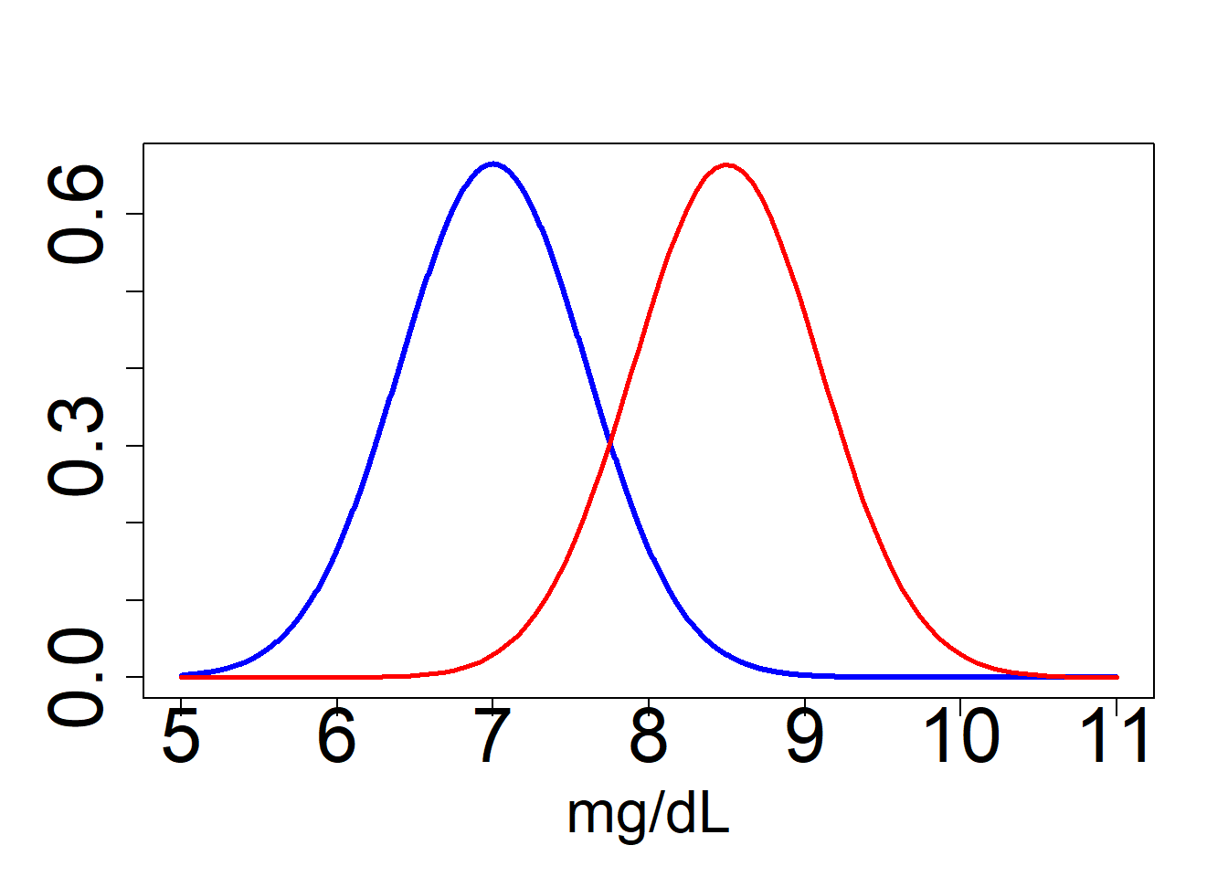
We need a threshold to decide between whether the athlete is doped or not in both situations (Decision of the anti-doping agency). mu=8.54 ng/ml
#function of probability under null hyphotesis and alternative hyphotesis
x<-seq(5,11,length=1000)
y<-dnorm(x,mean=7,sd=(2.4/sqrt(16)))
plot(x,y,type="l",lwd=3,col="blue",cex.axis=2.6,cex.lab=2, xlab = "mg/dL", ylab = "")
y2<-dnorm(x,mean=8.5,sd=(2.4/sqrt(16)))
curve(dnorm(x,mean=8.5,sd=(2.4/sqrt(16))),type="l",lwd=2.6,col="red",add=T)
# decision threshold
C=8.54
abline(v=C,lwd=2.6,col="black", lty=2)
legend("topleft",c("Normals","Formatge","Valor = XX ng/ml"),col=c("blue","red","black"),
lwd=2.6,bty="n",cex=1.5)
#POLÃGON DE PROBABILITAT
t<-seq(C,10,by=0.01)
x2 <- c(C,t,11)
y3 <- c(0,dnorm(t,mean=7,sd=2.4/sqrt(16)),0)
polygon(x2,y3,col="green")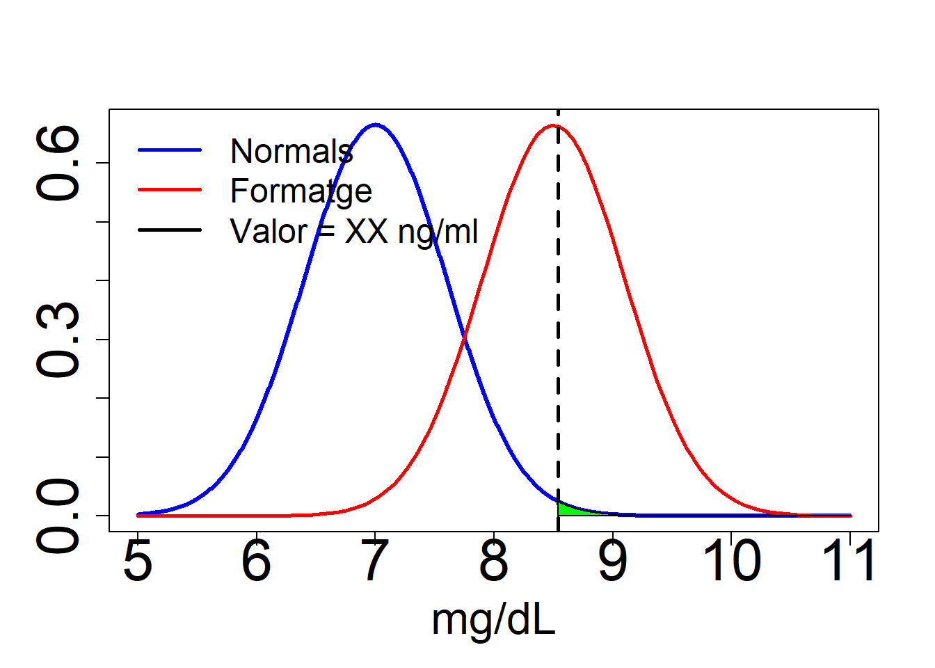
We wonder decide which scenario is more likely? We dismiss the null hypothesis and accept the alternative or not? We must be able to build a test based on probabilities for this decision.
To do this we take a sample of doped athletes and watch their level of hormone in blood and decided that this value is called critical value to decide among which are doped and not doped.
Let’s calculate the errors committed if you choose one or the other hypothesis: alfa and beta.
Alfa
C1 = 8 #Critical value decided in base of a sample of doped athletes
#Grà fic d' alfa ###############################################
x<-seq(5,10,length=1000)
y<-dnorm(x,mean=8.5,sd=(2.4/sqrt(16)))
plot(x,y,type="l",lwd=3,col="blue",cex.axis=2.6,cex.lab=2, xlab = "mg/dL", ylab = "")
y2<-dnorm(x,mean=7,sd=(2.4/sqrt(16)))
curve(dnorm(x,mean=7,sd=(2.4/sqrt(16))),type="l",lwd=2.6,col="red",add=T)
#llindar de decisió 8.54
abline(v=C1,lwd=2.6,col=3)
t<-seq(C1,10,by=0.01)
x2 <- c(C1,t,3)
y3 <- c(0,dnorm(t,mean=7,sd=2.4/sqrt(16)),0)
polygon(x2,y3,col="green")
text(C1,0.68,"C",cex=2)
#alfa
alfa = 1-pnorm(q=C1,mean=7,sd=(2.4/sqrt(16)))
alfa
## [1] 0.04779035Beta
#Grafic de beta ###################################################################
plot(x,y,type="l",lwd=2,col=2,cex.axis=2,cex.lab=2)
curve(dnorm(x,mean=7,sd=2.4/sqrt(16)),type="l",lwd=2,col=1,add=T)
abline(v=C1,lwd=2,col=3)
t2<-seq(6,C1,by=0.01)
x3 <- c(6,t2,C1)
y4 <- c(0,dnorm(t2,mean=8.5,sd=2.4/sqrt(16)),0)
polygon(x3,y4,col="orange")
text(C1,0.68,"C",cex=2)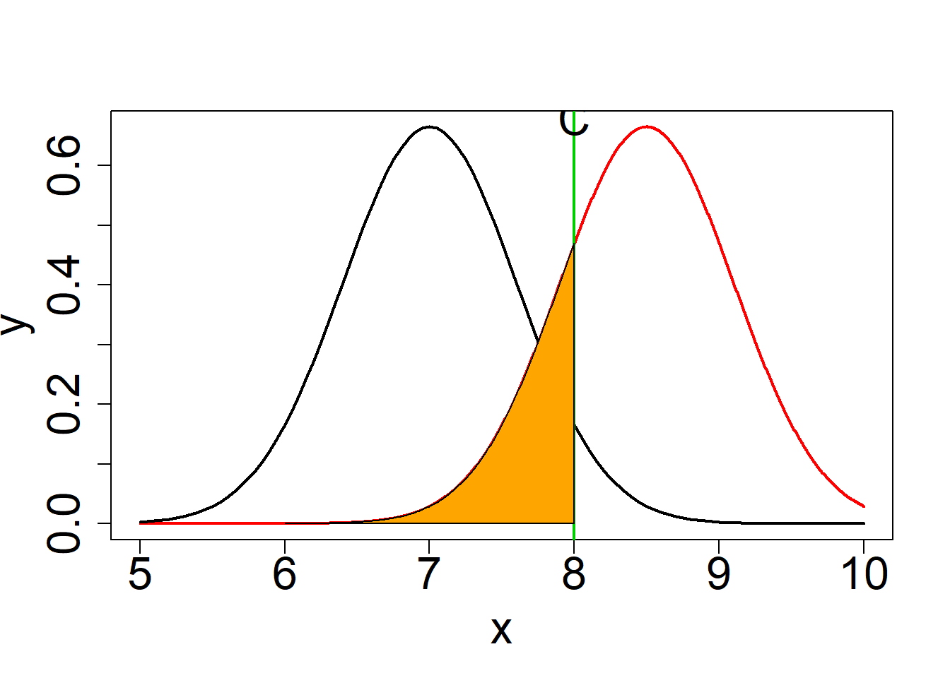
beta = pnorm(q=C1,mean=8.5,sd=(2.4/sqrt(16)))
beta
## [1] 0.2023284#probability of the errores type I and II
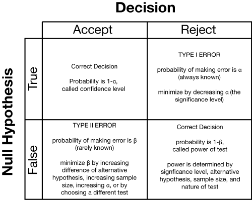
alfa## [1] 0.04779035beta## [1] 0.2023284We can talk about the errors. The statistical errors made if you choose one or the other hypothesis are those described in the following table:
The null hypothesis is either true or false. Unfortunately, we don’t know which is the case, and generally, we never will. It is important to realize that there is no probability that the null hypothesis is true or that it is false. Not knowing which is correct does not mean that a probability is involved. For example, if you are testing whether a potential mine has a greater gold concentration than that of break-even mine, the null hypothesis that your potential mine has a gold concentration no greater than a break-even mine is either true or it is false. There is no probability associated with these two cases (in a frequentist sense) because the gold is already in the ground - there is no possibility for chance because everything is already set. All we have is our own uncertainty about the null hypothesis.
This lack of knowledge about the null hypothesis is why we need to perform a statistical test: we want to use our data to make an inference about the null hypothesis. Specifically, we need to decide if we are going to act as if the null hypothesis is true or act as if it was false. From our hypothesis test, we therefore choose to either accept or reject the null hypothesis. If we accept the null hypothesis, we are stating that our data are consistent with the null hypothesis. If we reject the null hypothesis, we are stating that our data are such an unexpected outcome that they are inconsistent with the null hypothesis.
Our decision will change our behavior. If we reject the null hypothesis, we will act as if the null hypothesis is false, even though we do not know if that is the case. If we accept the null hypothesis, we will act as if the null hypothesis is true, even though we have not demonstrated that it is in fact true. This is a critical point: regardless of the results of our statistical test, we will never know if the null hypothesis is true or false.
Because we have two possibilities for the null hypothesis (true or false) and two possibilities for our decision (accept or reject), there are four possible scenarios. Two of these are correct decisions: we could accept a true null hypothesis or we could reject a false null hypothesis. The other two are errors. If we reject a true null hypothesis, we have committed a type I error. If we accept a false null hypothesis, we have made a type II error.
Each of these four possibilities has some probability of occurring. If the null hypothesis is true, there are only two possibilities: we will choose to accept the null hypothesis with probability of 1-, or we will reject it with probability of . If the null hypothesis is false, there are only two possibilities: we will choose to accept the null hypothesis with probability of ??, or we will reject it with probability of 1-. Because the probabilities are contingent on whether the null hypothesis is true or false, it is the probabilities in each row that sum to 100. The probabilities in each column are not constrained to sum to 100.
Because we don’t know the truth of a null hypothesis, we need to cover ourselves and lessen the chances of making both types of error. If the null hypothesis is true, we want to lessen our chances of making a type I error; in other words, we want to find ways to reduce alpha. If the the null hypothesis is false, we want to reduce our chances of making a type II error: we want to find ways to reduce beta. Because we do not know if the null hypothesis is true or false, we need to simultaneously keep the probabilities of both alpha and beta as small as possible.
Image origin http://daniellakens.blogspot.com/2016/12/why-type-1-errors-are-more-important.html 
(Figure and text from: )
Let’ s go to calculate alfa and beta in a test whith a small sample size (see at: ):
par(mfrow=c(2, 1))

# simulate Ho distribution for mean of small sample (n=20)
nullMean <- 4.5
nullStandardDeviation <- 1.0
smallSample <- 20
iterations <- 10000
smallSampleMeans <- replicate(iterations, mean(rnorm(smallSample, nullMean, nullStandardDeviation)))

alpha <- 0.05
xRange <- c(3, 6)

# plot the distribution of the mean and its critical value
hist(smallSampleMeans, breaks=100, col='gray', main='Hypothesized Mean n=20', xlab='mean', xlim=xRange)
smallSampleMeans <- sort(smallSampleMeans)
rightCutoff <- iterations * (1-alpha)
criticalValue <- smallSampleMeans[rightCutoff]
abline(v=criticalValue, col='blue', lwd=3)
text(criticalValue, 350, 'critical value', pos=4, col='blue')

# add an observed mean
observedMean <- 5.1
arrows(observedMean, 200, 5.1, 50, angle=20, length=0.15, lwd=3, col='red')
text(observedMean, 220, 'observed mean', pos=4, col='red')

# label alpha and 1-alpha
text(5.5, 100, expression(alpha), cex=2, pos=1, col='blue')
text(3.5, 100, expression(1-alpha), cex=2, pos=1, col='blue')

# simulate true distribution for mean of small sample (n=20); note: this is unknowable to us
trueMean <- 5.0
trueSd <- 1.0
trueSampleMeans <- replicate(iterations, mean(rnorm(smallSample, trueMean, trueSd)))

# plot the distribution, add critical value and observed mean
hist(trueSampleMeans, breaks=100, col='gray', main='True Mean (Unknowable)', xlab='mean', xlim=xRange)
criticalValue <- smallSampleMeans[rightCutoff]
abline(v=criticalValue, col='blue', lwd=3)
arrows(observedMean, 200, 5.1, 50, angle=20, length=0.15, lwd=3, col='red')

# label beta and 1-beta
text(5.5, 300, expression(1-beta), cex=2, pos=1, col='blue')
text(3.5, 300, expression(beta), cex=2, pos=1, col='blue')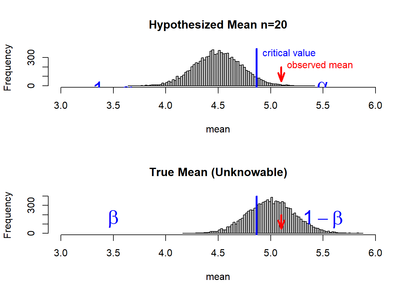
# Be aware of the magic numbers used in plotting arrows and
# and text labels. If you modify the code, you will likely
# need to change these numbers
p-value
In frequentist statistics, the p-value is a function of the observed sample results (a test statistic) relative to a statistical model, which measures how extreme the observation is. Statistical hypothesis tests making use of p-values are commonly used in many fields of science

The p-value is used in the context of null hypothesis testing in order to quantify the idea of statistical significance of evidence.[a] Null hypothesis testing is a reductio ad absurdum argument adapted to statistics. In essence, a claim is shown to be valid by demonstrating the improbability of the consequence that results from assuming the counter-claim to be true.
See more information about distribution at this link:
see link at: https://upload.wikimedia.org/wikipedia/commons/thumb/8/89/P_values.png/475px-P_values.png
We look at the steps necessary to calculate the p value for a particular test (an example). In the interest of simplicity we only look at a two sided test, and we focus on one example. Here we want to show that the mean is not close to a fixed value, a. Ho:\(mu_x\)=a, Ha:\(mu_x\)<>a,
The p value is calculated for a particular sample mean. Here we assume that we obtained a sample mean, x and want to find its p value. It is the probability that we would obtain a given sample mean that is greater than the absolute value of its Z-score or less than the negative of the absolute value of its Z-score.
For the special case of a normal distribution we also need the standard deviation. We will assume that we are given the standard deviation and call it s. The calculation for the p value can be done in several of ways. We will look at two ways here. The first way is to convert the sample means to their associated Z-score. The other way is to simply specify the standard deviation and let the computer do the conversion. At first glance it may seem like a no brainer, and we should just use the second method. Unfortunately, when using the t-distribution we need to convert to the t-score, so it is a good idea to know both ways.
We first look at how to calculate the p value using the Z-score. The Z-score is found by assuming that the null hypothesis is true, subtracting the assumed mean, and dividing by the theoretical standard deviation. Once the Z-score is found the probability that the value could be less the Z-score is found using the pnorm command.
This is not enough to get the p value. If the Z-score that is found is positive then we need to take one minus the associated probability. Also, for a two sided test we need to multiply the result by two. Here we avoid these issues and insure that the Z-score is negative by taking the negative of the absolute value.
EXAMPLE We now look at a specific example. Let’ s go to do a z test to compare an observed mean of 7 with the waited mean of 5 when the stardar desviation is known in the population and has a value of 2 In the example below we will use a value of a of 5, a standard deviation of 2, and a sample size of 20. We then find the p value for a sample mean of 7:
 a <- 5 #population mean
 s <- 2 #standart desviation
 n <- 20 #sample size
 xbar <- 7 #observed mean in the samples
 z <- (xbar-a)/(s/sqrt(n)) #Z statistic <-> Z experimental
 z #<Z experimental
## [1] 4.472136 #Calculate the p-value using the normal distribution with pnorm()
2*pnorm(-abs(z))## [1] 7.744216e-06
Why p-value is 0? Where is the Z experimental in the normal function?
#Where the point 4 is in the right tail
set.seed(3000)
xseq<-seq(-4,4,.01)
densities<-dnorm(xseq, 0,1)
cumulative<-pnorm(xseq, 0, 1)
randomdeviates<-rnorm(1000,0,1)

par(mfrow=c(1,3), mar=c(3,4,4,2))

plot(xseq, densities, col="darkgreen",xlab="", ylab="Density", type="l",lwd=2, cex=2, main="PDF of Standard Normal", cex.axis=.8)

plot(xseq, cumulative, col="darkorange", xlab="", ylab="Cumulative Probability",type="l",lwd=2, cex=2, main="CDF of Standard Normal", cex.axis=.8)

hist(randomdeviates, main="Random draws from Std Normal", cex.axis=.8, xlim=c(-4,4))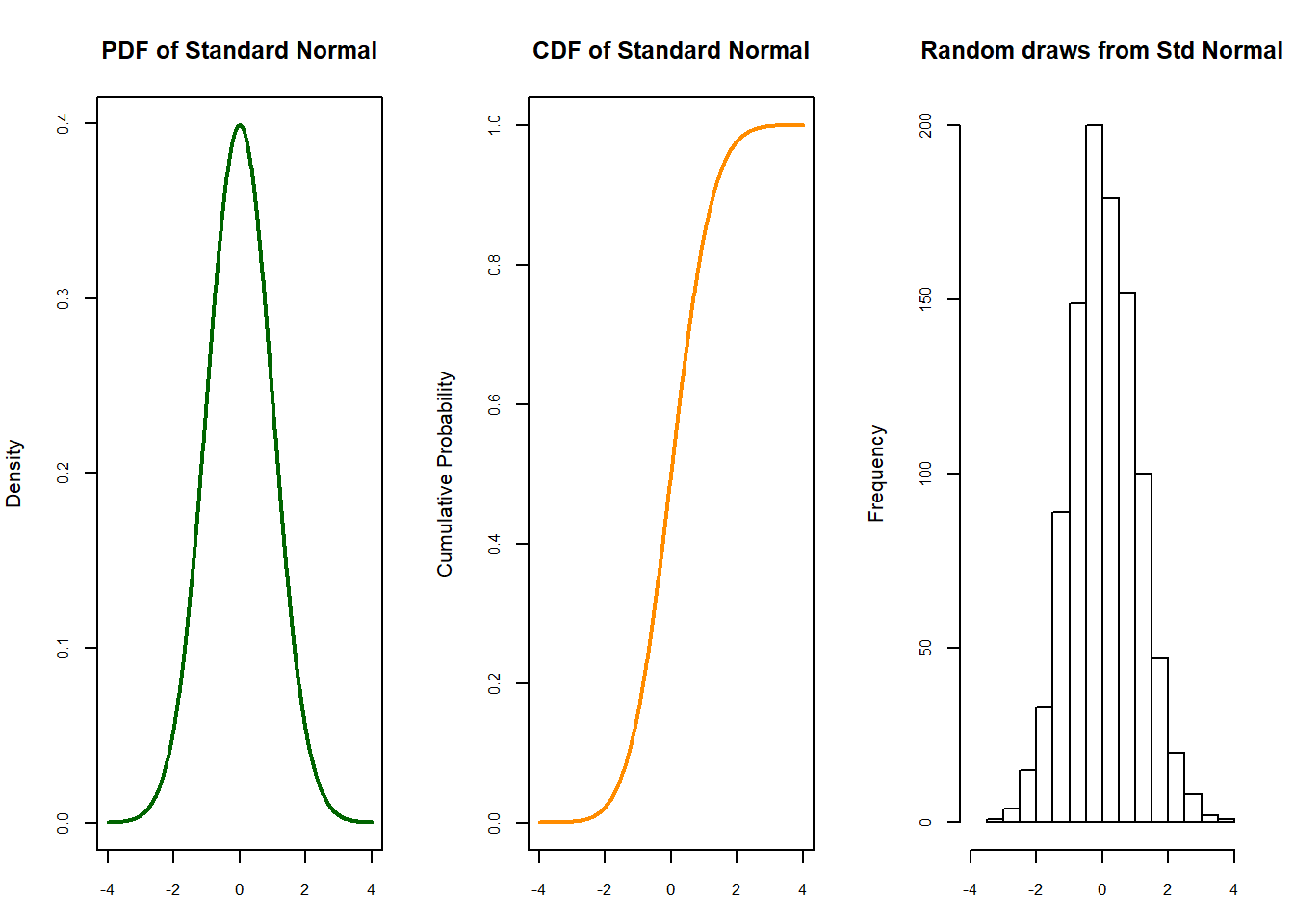
EXAMPLES OF HYPOTHESIS TEST
Hypothesis Testing Steps
Define the Problem
State the Objectives
Establish the Hypothesis (left-tailed, right-tailed, or two tailed test).
State the Null Hypothesis (Ho)
State the Alternative Hypothesis (Ha)
Select the appropriate statistical test
State the alpha-risk (a) level
State the beta-risk (ß) level
Establish the Effect Size
Create Sampling Plan, determine sample size
Gather samples
Collect and record data
Calculate the test statistic
Determine the p-value
Types of test in fuction of data:

test for comparison of means:
Z test
A first example
Test mean parameter a one population in a normal distribution population. Sigma (\(\sigma^{2}\)) is known and n large.
See more information about distribution at this link:
Suppose that the normal mean value of a biochemical marker in the bood is 14.6 U. In a sample of 35 patients the value of this biochemical marker is 15.4U. Assume the population standard deviation is 2.5 kg. At .05 significance level. Can we reject the null hypothesis that the mean biochemical marker does not differ from the normal value?
 xbar = 14.6            # sample mean
 mu0 = 15.4             # hypothesized value
 sigma = 2.5            # population standard deviation
 n = 35                 # sample size
 z = (xbar-mu0)/
   (sigma/sqrt(n))      # calculate the Z experimental
 # and the result of the Z statistic (Z experimental) is:
 z                      # test statistic
## [1] -1.893146 #Probability under the null hypothesis
2*pnorm(z)## [1] 0.05833852A second example.
We start out with a one-sample Z-test to check the hypothesis to compare if mean = 5 or not:
H0 : \(\mu\) = 5
H1 : \(\mu\) <> 5
Start by typing z.test.
library(BSDA)## Warning: package 'BSDA' was built under R version 3.4.3## Loading required package: lattice##
## Attaching package: 'BSDA'## The following object is masked from 'package:datasets':
##
## Orange#lets go to use the instruction z.test
x <- rnorm(47, 6, 1) #simulate a sample with a mean = 6 and a stv = 1 (n=47)
z.test(x, y = NULL,alternative = "two.sided",mu = 5,sigma.x=1,conf.level = 0.95)##
## One-sample z-Test
##
## data: x
## z = 7.5708, p-value = 3.709e-14
## alternative hypothesis: true mean is not equal to 5
## 95 percent confidence interval:
## 5.818428 6.390208
## sample estimates:
## mean of x
## 6.104318What was the result? Can you reject the null hypothesis or not? Calculate the confidence interval by hand and compare.
Repeat the procedure but change alternative to greater and less. Did the results change? What can we say about the null hypothesis?
#lets go to use the instruction z.test
z.test(x, y = NULL,alternative = "greater",mu = 5,sigma.x=1,conf.level = 0.95)
##
## One-sample z-Test
##
## data: x
## z = 7.5708, p-value = 1.854e-14
## alternative hypothesis: true mean is greater than 5
## 95 percent confidence interval:
## 5.864391 NA
## sample estimates:
## mean of x
## 6.104318z.test(x, y = NULL,alternative = "less",mu = 5,sigma.x=1,conf.level = 0.95)##
## One-sample z-Test
##
## data: x
## z = 7.5708, p-value = 1
## alternative hypothesis: true mean is less than 5
## 95 percent confidence interval:
## NA 6.344244
## sample estimates:
## mean of x
## 6.104318
Repeat the procedure for another data set. What can you say?
T-Test: one population examples
Sigma (\(\sigma^{2}\)) is unknown.
Remenber use this distribution when estimating the mean of a normally distributed population in situations where the sample size is small and population standard deviation is unknown.
FIRST EXAMPLE
PAGINA 167-libro de problemas de Cuadras: Set of cans and its capacityHo: \(\mu\) = 1000
Ho: \(\mu\) <> 1000
lets go to compare the expected weight of a set of cans with the observed weight of a sample set
weight_cans <- c(995, 992, 1005, 998, 1000)

# A sample
# help(t.test)

summary(weight_cans)
## Min. 1st Qu. Median Mean 3rd Qu. Max.
## 992 995 998 998 1000 1005#solution using t.test
t.test(weight_cans, alternative="two.sided", mu=1000, conf.level = 0.95)##
## One Sample t-test
##
## data: weight_cans
## t = -0.90351, df = 4, p-value = 0.4173
## alternative hypothesis: true mean is not equal to 1000
## 95 percent confidence interval:
## 991.8541 1004.1459
## sample estimates:
## mean of x
## 9982ND EXAMPLE
Time (months) until Relapse in Tuberculosis Treatment in months
The data:
  Time_until_Relapse <- c(0.2, 0.2, 0.2, 0.2, 0.7, 0.7, 0.7,
0.8, 0.8, 0.8, 0.8, 0.8, 0.8, 1.2, 1.8, 1.8, 1.8, 1.8, 1.8, 1.8, 1.8, 1.8,
2.0, 2.0, 2.0, 2.0, 2.0, 2.0, 2.0, 2.0, 2.0, 3.1, 3.1, 3.1, 3.1, 3.1, 3.1,
3.1, 3.1, 3.1, 3.1, 3.1, 3.1, 3.1, 3.1, 3.1, 3.1, 3.1, 3.4, 3.4, 3.4, 3.4, 3.4)
We need to check if the time until relapse is greater than 2 monts or not.
The hypothesis:
\(\mu\) = 2
Ho: \(\mu\) > 2
And the solution:
# one sample
# help(t.test)

summary(Time_until_Relapse)
## Min. 1st Qu. Median Mean 3rd Qu. Max.
## 0.200 1.200 2.000 2.094 3.100 3.400#solution using t.test:
t.test(Time_until_Relapse,alternative="greater",mu=2)##
## One Sample t-test
##
## data: Time_until_Relapse
## t = 0.65297, df = 52, p-value = 0.2583
## alternative hypothesis: true mean is greater than 2
## 95 percent confidence interval:
## 1.852384 Inf
## sample estimates:
## mean of x
## 2.09434hist(Time_until_Relapse)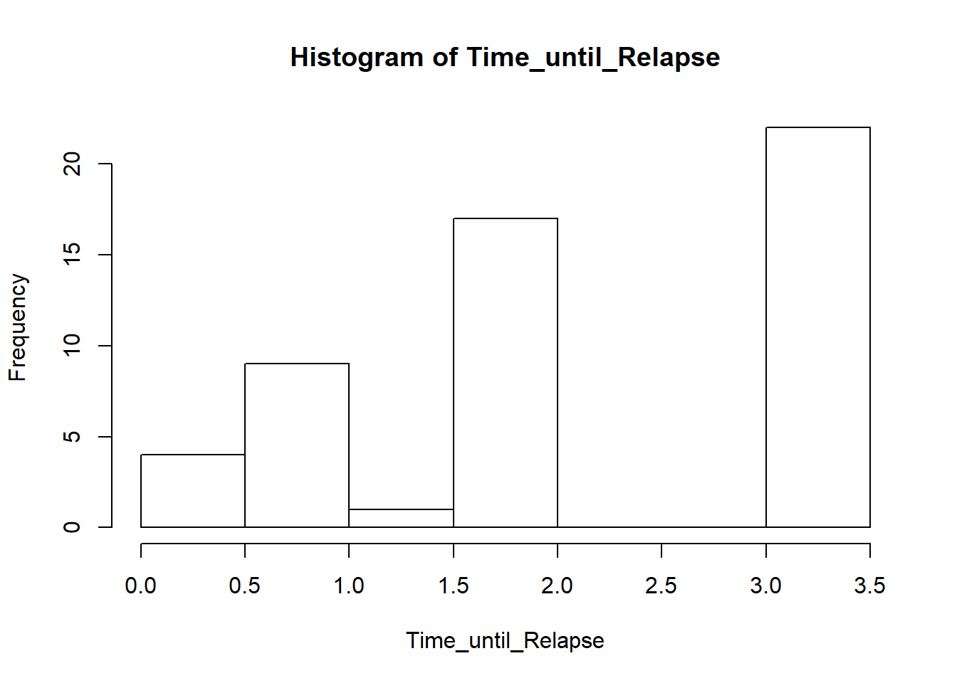
#?histogram\(\sigma^{2}\) - test
The \(\sigma^{2}\) test is used for testing hypotheses about the standard deviation of one population. We start by testing the hypothesis with the example of hypothesis:
H0 : \(\sigma^{2}_x\) = 1
H1 : \(\sigma^{2}_x\) <> 1
Use the \(\sigma^{2}_x\) test:
library(TeachingDemos)## Warning: package 'TeachingDemos' was built under R version 3.4.3##
## Attaching package: 'TeachingDemos'## The following object is masked from 'package:BSDA':
##
## z.testx<-c(2, 6, 5, 2, 8)
var(x) #variance of x## [1] 6.8sigma.test(x, sigma = 1, alternative ="two.sided", conf.level = 0.95) #add the confidence interval for the variance##
## One sample Chi-squared test for variance
##
## data: x
## X-squared = 27.2, df = 4, p-value = 3.622e-05
## alternative hypothesis: true variance is not equal to 1
## 95 percent confidence interval:
## 2.440932 56.149789
## sample estimates:
## var of x
## 6.8Play around with different values on sigma and conf.level. What can you say? Calculate the confidence interval by hand and compare.
F-Test
Now we want to do a two-sample test about the variances in our data sets. We want to test the hypothesis:H0 :\(\sigma^{2}_x\) = \(\sigma^{2}_y\)
H1 :\(\sigma^{2}_x\) <> \(\sigma^{2}_y\)
Type var.test and then
y<-c(2, 2, 3, 3, 4)
x<-c(2, 16, 15, 12, 8)
summary(x)
## Min. 1st Qu. Median Mean 3rd Qu. Max.
## 2.0 8.0 12.0 10.6 15.0 16.0summary(y)## Min. 1st Qu. Median Mean 3rd Qu. Max.
## 2.0 2.0 3.0 2.8 3.0 4.0var.test(x, y, ratio = 1, alternative = "two.sided", conf.level = 0.95)##
## F test to compare two variances
##
## data: x and y
## F = 46.857, num df = 4, denom df = 4, p-value = 0.002583
## alternative hypothesis: true ratio of variances is not equal to 1
## 95 percent confidence interval:
## 4.87865 450.04083
## sample estimates:
## ratio of variances
## 46.85714Conclusion? Calculate the confidence interval by hand and compare.
T-Test: two populations
See at Probabilidad y Estad?stica. Cuadras p?gina 167.
12 elderly patients who are admitted to a hospital having trouble sleeping problems. They want to test whether a drug helps them sleep more.
hours.sleeping.basal <- c(7, 5, 8, 8.5, 6, 7, 8) #n=7
hours.sleeping.after.drug <- c(9, 8.5, 9.5, 10, 8) #n=5

summary(hours.sleeping.basal)
## Min. 1st Qu. Median Mean 3rd Qu. Max.
## 5.000 6.500 7.000 7.071 8.000 8.500summary(hours.sleeping.after.drug) ## Min. 1st Qu. Median Mean 3rd Qu. Max.
## 8.0 8.5 9.0 9.0 9.5 10.0 # Ho: m1 = m2 frente a H1: m1 < m2
# help(t.test)
# help(var.test)
var.test(hours.sleeping.basal, hours.sleeping.after.drug, ratio=1, alternative = "two.sided")##
## F test to compare two variances
##
## data: hours.sleeping.basal and hours.sleeping.after.drug
## F = 2.4571, num df = 6, denom df = 4, p-value = 0.4035
## alternative hypothesis: true ratio of variances is not equal to 1
## 95 percent confidence interval:
## 0.2671588 15.3010246
## sample estimates:
## ratio of variances
## 2.457143t.test(hours.sleeping.basal, hours.sleeping.after.drug, var.equal = TRUE, alternative = "less") ##
## Two Sample t-test
##
## data: hours.sleeping.basal and hours.sleeping.after.drug
## t = -3.0431, df = 10, p-value = 0.006198
## alternative hypothesis: true difference in means is less than 0
## 95 percent confidence interval:
## -Inf -0.7799334
## sample estimates:
## mean of x mean of y
## 7.071429 9.000000#alternative = c("two.sided", "less", "greater"),
# mu = 0, paired = FALSE, var.equal = FALSE,
# conf.level = 0.95, ...)T Test: paired samples
  #a biochemical marker level basal and after a treatment
basal <- c(190, 203, 185, 212, 240, 197, 189, 205, 222, 191, 203, 210)
after.treatment <- c(202, 180, 176, 191, 165, 193, 182, 213, 187, 170, 175, 179)
# two paired samples
# help(t.test)
#solution:
tResult <- t.test(basal, after.treatment, var.equal = TRUE, paired = TRUE)
tResult##
## Paired t-test
##
## data: basal and after.treatment
## t = 2.9425, df = 11, p-value = 0.01339
## alternative hypothesis: true difference in means is not equal to 0
## 95 percent confidence interval:
## 4.914148 34.085852
## sample estimates:
## mean of the differences
## 19.5Chi-square test
Chi-Square Test of Independence: First example
  taula <- c(100, 71, 29, 146, 32, 17, 149, 28, 16, 146, 37, 17, 147, 33, 18)
taula <- matrix(taula,ncol=5)
rownames(taula) <- c("no infected","slightly infected","severely infected")
colnames(taula) <- c("P","A","B","C","D") #treatment, P = Placebo
taula
## P A B C D
## no infected 100 146 149 146 147
## slightly infected 71 32 28 37 33
## severely infected 29 17 16 17 18 # frequencies marginals
f.files <- apply(taula,1,sum)
f.col <- apply(taula,2,sum)
n <- sum(taula) # sample size
# table of expected frequencies
E <- outer(f.files,f.col)/n
round(E, 2)## P A B C D
## no infected 139.55 136.06 134.67 139.55 138.16
## slightly infected 40.77 39.75 39.34 40.77 40.36
## severely infected 19.68 19.18 18.99 19.68 19.48 khi.quadr <- sum((taula-E)^2 / E)
p.valor <- pchisq(khi.quadr,df=8,lower.tail=F) # p.valor < 0.05
khi.quadr; p.valor## [1] 48.82569## [1] 6.866105e-08## Chi-Square Test
chisq.test(taula)##
## Pearson's Chi-squared test
##
## data: taula
## X-squared = 48.826, df = 8, p-value = 6.866e-08Chi-Square Test of Independence: 2nd example
  taula <- c(12, 14, 11, 0, 13, 18, 27, 9, 11, 11, 29, 16, 0, 0, 13, 12)
taula <- matrix(taula,ncol=4)
rownames(taula) <- c("no fumen","1-5","6-30","31-45")
colnames(taula) <- c("10-19","20-29","30-39","40-49")
taula
## 10-19 20-29 30-39 40-49
## no fumen 12 13 11 0
## 1-5 14 18 11 0
## 6-30 11 27 29 13
## 31-45 0 9 16 12 ## Test directe
chisq.test(taula) # Warning message: Chi-squared approximation may be incorrect## Warning in chisq.test(taula): Chi-squared approximation may be incorrect##
## Pearson's Chi-squared test
##
## data: taula
## X-squared = 42.316, df = 9, p-value = 2.877e-06 # frequencies marginals
f.files <- apply(taula,1,sum)
f.col <- apply(taula,2,sum)
n <- sum(taula) # mida de la mostra
# taula de frequencies esperades
E <- outer(f.files,f.col)/n
round(E, 2) # Hem d'ajuntar les dues darreres columnes## 10-19 20-29 30-39 40-49
## no fumen 6.80 12.31 12.31 4.59
## 1-5 8.12 14.70 14.70 5.48
## 6-30 15.10 27.35 27.35 10.20
## 31-45 6.98 12.65 12.65 4.72taula.nova <- round(E, 2)
chisq.test(taula.nova)## Warning in chisq.test(taula.nova): Chi-squared approximation may be
## incorrect##
## Pearson's Chi-squared test
##
## data: taula.nova
## X-squared = 7.8901e-06, df = 9, p-value = 1Chi-Square Test of Independence - MORE EXAMPLES
  taula <- c(12, 14, 11, 0, 13, 18, 27, 9, 11, 11, 29, 16, 0, 0, 13, 12)
taula <- matrix(taula,ncol=4)
rownames(taula) <- c("no fumen","1-5","6-30","31-45")
colnames(taula) <- c("10-19","20-29","30-39","40-49")
taula
## 10-19 20-29 30-39 40-49
## no fumen 12 13 11 0
## 1-5 14 18 11 0
## 6-30 11 27 29 13
## 31-45 0 9 16 12 ## Test directe
chisq.test(taula) # Warning message: Chi-squared approximation may be incorrect## Warning in chisq.test(taula): Chi-squared approximation may be incorrect##
## Pearson's Chi-squared test
##
## data: taula
## X-squared = 42.316, df = 9, p-value = 2.877e-06 # frequencies marginals
f.files <- apply(taula,1,sum)
f.col <- apply(taula,2,sum)
n <- sum(taula) # mida de la mostra # taula de frequencies esperades
E <- outer(f.files,f.col)/n
round(E, 2) # Hem d'ajuntar les dues darreres columnes## 10-19 20-29 30-39 40-49
## no fumen 6.80 12.31 12.31 4.59
## 1-5 8.12 14.70 14.70 5.48
## 6-30 15.10 27.35 27.35 10.20
## 31-45 6.98 12.65 12.65 4.72taula.nova <- round(E, 2)
chisq.test(taula.nova)## Warning in chisq.test(taula.nova): Chi-squared approximation may be
## incorrect##
## Pearson's Chi-squared test
##
## data: taula.nova
## X-squared = 7.8901e-06, df = 9, p-value = 1 # We then compute the critical values at .05 significance level.
alpha = .05
z.half.alpha = qnorm(1-alpha/2)
c(-z.half.alpha, z.half.alpha) ## [1] -1.959964 1.959964# The test statistic -1.8931 lies between the critical values -1.9600 and 1.9600.
# Hence, at .05 significance level, we do not reject the null hypothesis that the mean does not differ from normal population. #Instead of using the critical value, we apply the pnorm function to compute the two-tailed
#p-value of the test statistic. It doubles the lower tail p-value
#as the sample mean is less than the hypothesized value.
#Since it turns out to be greater than the .05 significance level, we do not reject the null hypothesis that ? = 15.4.
pval = 2 * pnorm(z) # lower tail
pval # two-tailed p-value ## [1] 0.05833852Goodness of fit Chi-Square test: Test the normality of data
Problema 9.3 de Cuadras vol. 2
  talls <- seq(54.99,57.49,by=0.25)
freq <- c(2, 25, 18, 30, 23, 41, 23, 28, 17, 24, 19)
n <- sum(freq)
# Un grafic per acompanyar les dades
mc <- talls-0.25/2 # Marques de classe
dades <- rep(mc,freq)
talls.p <- c(54.74,talls)
dades## [1] 54.865 54.865 55.115 55.115 55.115 55.115 55.115 55.115 55.115 55.115
## [11] 55.115 55.115 55.115 55.115 55.115 55.115 55.115 55.115 55.115 55.115
## [21] 55.115 55.115 55.115 55.115 55.115 55.115 55.115 55.365 55.365 55.365
## [31] 55.365 55.365 55.365 55.365 55.365 55.365 55.365 55.365 55.365 55.365
## [41] 55.365 55.365 55.365 55.365 55.365 55.615 55.615 55.615 55.615 55.615
## [51] 55.615 55.615 55.615 55.615 55.615 55.615 55.615 55.615 55.615 55.615
## [61] 55.615 55.615 55.615 55.615 55.615 55.615 55.615 55.615 55.615 55.615
## [71] 55.615 55.615 55.615 55.615 55.615 55.865 55.865 55.865 55.865 55.865
## [81] 55.865 55.865 55.865 55.865 55.865 55.865 55.865 55.865 55.865 55.865
## [91] 55.865 55.865 55.865 55.865 55.865 55.865 55.865 55.865 56.115 56.115
## [101] 56.115 56.115 56.115 56.115 56.115 56.115 56.115 56.115 56.115 56.115
## [111] 56.115 56.115 56.115 56.115 56.115 56.115 56.115 56.115 56.115 56.115
## [121] 56.115 56.115 56.115 56.115 56.115 56.115 56.115 56.115 56.115 56.115
## [131] 56.115 56.115 56.115 56.115 56.115 56.115 56.115 56.115 56.115 56.365
## [141] 56.365 56.365 56.365 56.365 56.365 56.365 56.365 56.365 56.365 56.365
## [151] 56.365 56.365 56.365 56.365 56.365 56.365 56.365 56.365 56.365 56.365
## [161] 56.365 56.365 56.615 56.615 56.615 56.615 56.615 56.615 56.615 56.615
## [171] 56.615 56.615 56.615 56.615 56.615 56.615 56.615 56.615 56.615 56.615
## [181] 56.615 56.615 56.615 56.615 56.615 56.615 56.615 56.615 56.615 56.615
## [191] 56.865 56.865 56.865 56.865 56.865 56.865 56.865 56.865 56.865 56.865
## [201] 56.865 56.865 56.865 56.865 56.865 56.865 56.865 57.115 57.115 57.115
## [211] 57.115 57.115 57.115 57.115 57.115 57.115 57.115 57.115 57.115 57.115
## [221] 57.115 57.115 57.115 57.115 57.115 57.115 57.115 57.115 57.115 57.115
## [231] 57.115 57.365 57.365 57.365 57.365 57.365 57.365 57.365 57.365 57.365
## [241] 57.365 57.365 57.365 57.365 57.365 57.365 57.365 57.365 57.365 57.365# Mitjana i desviacio estandard
# mitjana <- sum(mc*freq)/n
# desv <- sqrt(sum(mc^2*freq)/n - mitjana^2)
mitjana <- 56.17
desv <- 0.69
hist(dades,breaks=talls.p) # histograma de frequencies absolutes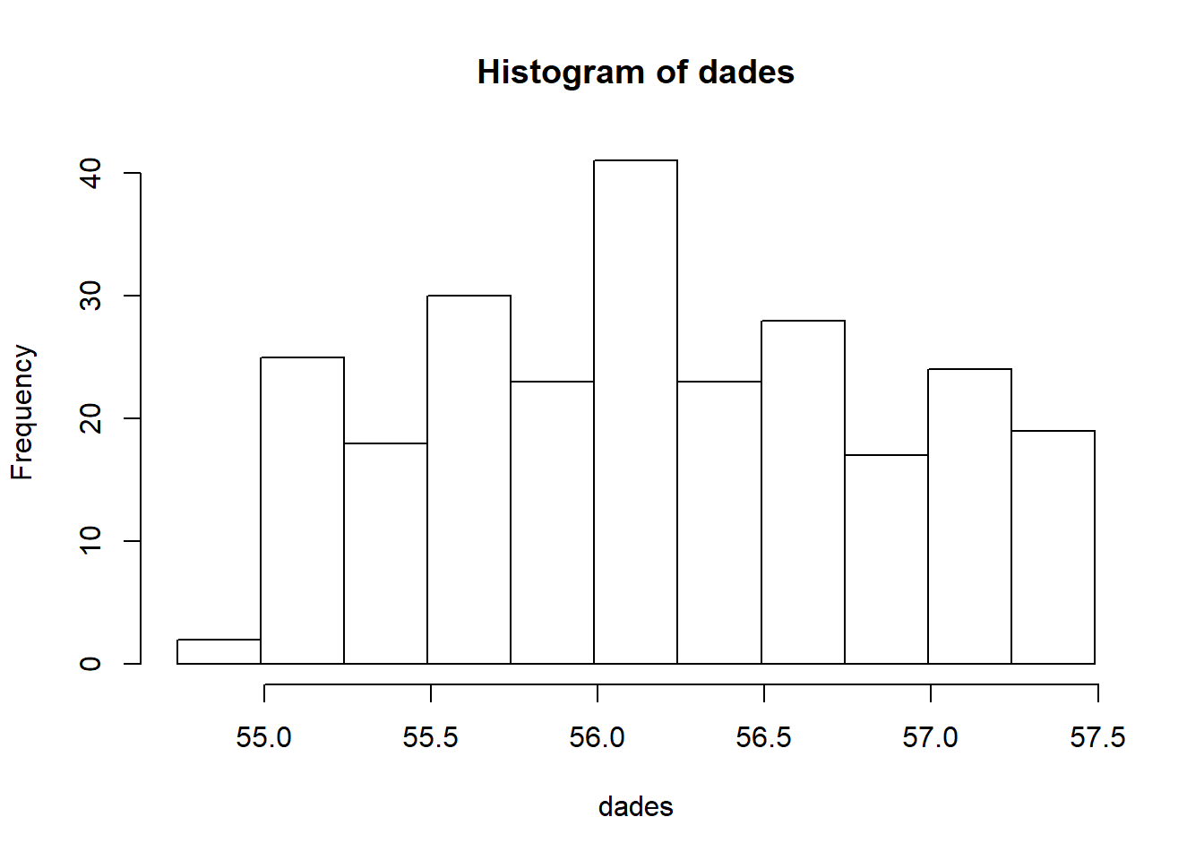
hist(dades, breaks=talls.p, prob=T) # histograma de frequencies relatives
curve(dnorm(x, mean=mitjana, sd=desv),add=T)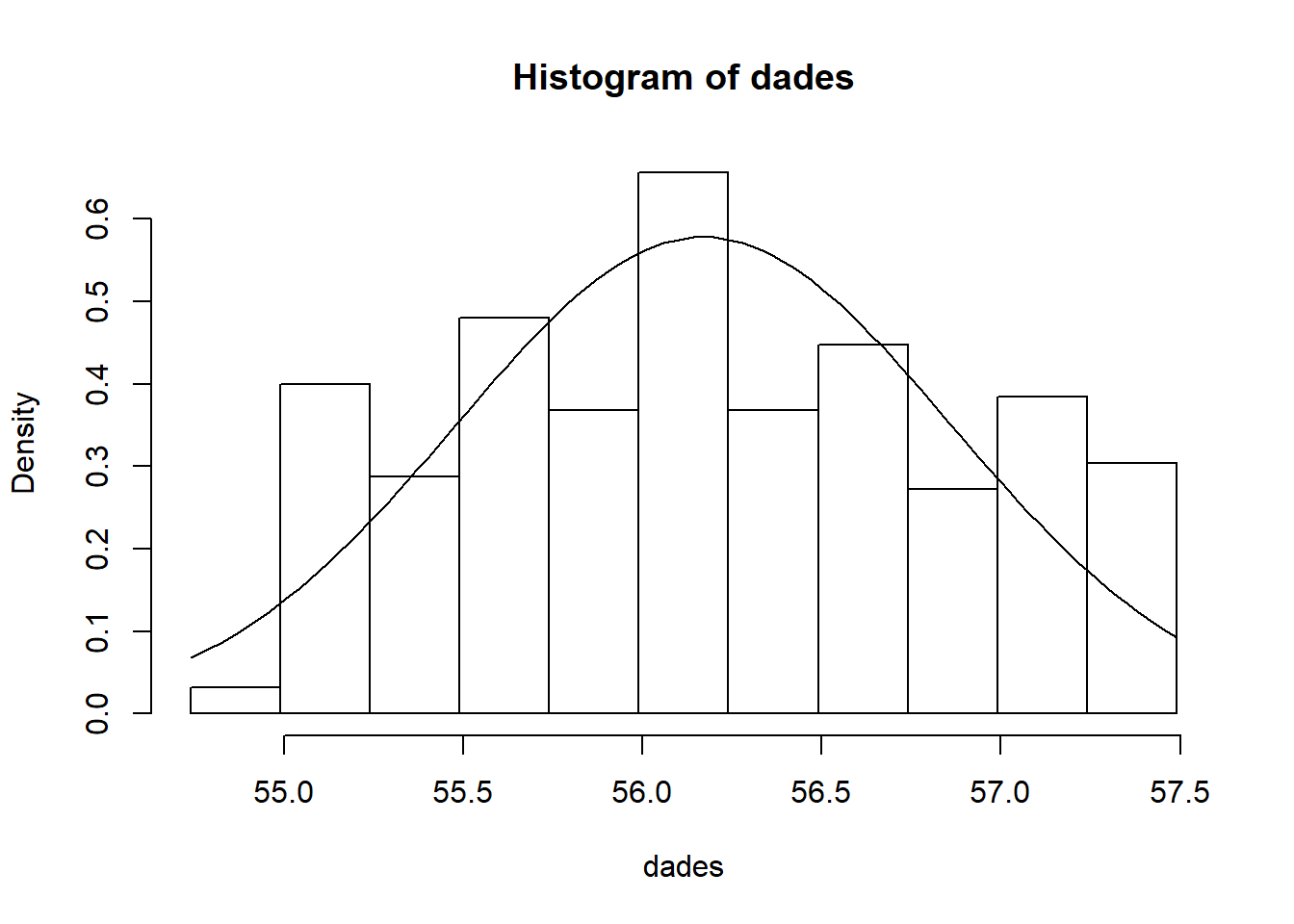
  # Funcio de distribucio normal

cua.esquerra <- pnorm(talls,mean=mitjana,sd=desv)
prob <- c(cua.esquerra[1],diff(cua.esquerra)) # probabilitats dels 11 intervals
sum(prob) # no suma 1
## [1] 0.9721288prob[11] <- 1-cua.esquerra[10] # millor ara
sum(prob) # ara si## [1] 1 # Test khi quadrat de bondat d'ajust
chisq.test(freq,p=prob) ##
## Chi-squared test for given probabilities
##
## data: freq
## X-squared = 40.712, df = 10, p-value = 1.269e-05POWER AND SAMPLE SIZE IN THE DESIGN OF THE EXPERIMENTS
Performing power analysis and sample size estimation is an important aspect of experimental design, because without these calculations, sample size may be too high or too low. If sample size is too low, the experiment will lack the precision to provide reliable answers to the questions it is investigating. If sample size is too large, time and resources will be wasted, often for minimal gain.
In some power analysis software programs, a number of graphical and analytical tools are available to enable precise evaluation of the factors affecting power and sample size in many of the most commonly encountered statistical analyses. This information can be crucial to the design of a study that is cost-effective and scientifically useful.
See more information at this link:
Sample size examples: compare means
Power analysis in compare mean of two populations
Calculating specific values of power, sample size or effect size can be illuminating with regard to the statistical restrictions on experimental design and analysis. But frequently a graph tells the story more completely and succinctly. Here we show how to draw power, sample size, and effect size curves using the above functions in R:
#Power curve for t-test with delta = 1
nvals <- seq(2, 100, length.out=200)
powvals <- sapply(nvals, function (x) power.t.test(n=x, delta=1)$power)
plot(nvals, powvals, xlab="n", ylab="power",
main="Power curve for\n t-test with delta = 1",
lwd=2, col="red", type="l")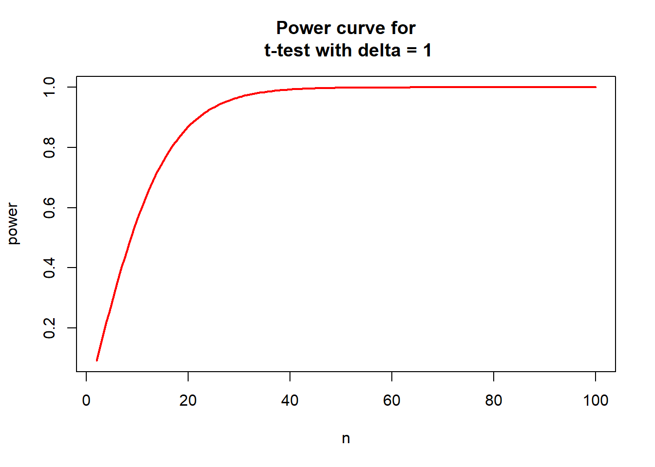
(More information at: )
of our effect size, we can also alter delta to see the effect of both effect size and sample size on power:
#Power Curve for\nt-test with varying delta
deltas <- c(0.2, 0.4, 0.8)
plot(nvals, seq(0,1, length.out=length(nvals)), xlab="n", ylab="power",
main="Power Curve for\nt-test with varying delta", type="n")
for (i in 1:3) {
powvals <- sapply(nvals, function (x) power.t.test(n=x, delta=deltas[i])$power)
lines(nvals, powvals, lwd=2, col=i)
}
legend("topleft", lwd=2, col=1:3, legend=c("0.2", "0.4", "0.8"))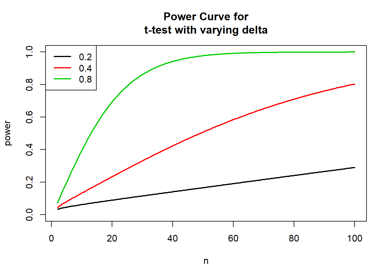
Sample size: compare mean of two populations, a first example
More examples at:
library(pwr)

#calculate the sample size in our "classical example T-test 2 populations". H1: "two.sided"
yA <- c(0.92, 1.29, 1, 1.5, 1.25, 1.54, 1.26, 1.71, 1.28) #first population
yB <- c(1.16, 1.43, 1.8, 1.5, 1.57, 1.75) #second population
mean(yA); sd(yA, na.rm = FALSE)
## [1] 1.305556## [1] 0.2511031mean(yB); sd(yB, na.rm = FALSE)## [1] 1.535## [1] 0.2326156yA_B <- c(0.92, 1.29, 1, 1.5, 1.25, 1.54, 1.26, 1.71, 1.28, 1.16, 1.43, 1.8, 1.5, 1.57, 1.75)
sd(yA_B, na.rm = FALSE) #join sdv## [1] 0.2624736# T test two populations in the case of H1: "two.sided"
tResult <- t.test(yA, yB, var.equal = TRUE)
tResult##
## Two Sample t-test
##
## data: yA and yB
## t = -1.783, df = 13, p-value = 0.09793
## alternative hypothesis: true difference in means is not equal to 0
## 95 percent confidence interval:
## -0.50744650 0.04855761
## sample estimates:
## mean of x mean of y
## 1.305556 1.535000mean1 <- mean(yA)
mean2 <- mean(yB)
sigma <- sd(yA_B, na.rm = FALSE)
delta= (mean1-mean2) / sigma
delta## [1] -0.8741621pwr.t.test(d=delta,power=0.8,sig.level=0.05,type="two.sample",alternative="two.sided")##
## Two-sample t test power calculation
##
## n = 21.54634
## d = 0.8741621
## sig.level = 0.05
## power = 0.8
## alternative = two.sided
##
## NOTE: n is number in *each* grouppwr.t.test(d=delta,n=9,sig.level=0.05,type="two.sample",alternative="two.sided")##
## Two-sample t test power calculation
##
## n = 9
## d = 0.8741621
## sig.level = 0.05
## power = 0.41426
## alternative = two.sided
##
## NOTE: n is number in *each* groupWhat is the problem here? Explain it!!
Sample size: compare mean of two populations, 2nd example
(see more sample size examples from UCLA at: )
See examples at: and
Example 1. A company markets an eight week long weight loss program and claims that at the end of the program on average a participant will have lost 5 pounds. On the other hand, you have studied the program and you believe that their program is scientifically unsound and shouldn’t work at all. With some limited funding at hand, you want test the hypothesis that the weight loss program does not help people lose weight. Your plan is to get a random sample of people and put them on the program. You will measure their weight at the beginning of the program and then measure their weight again at the end of the program. Based on some previous research, you believe that the standard deviation of the weight difference over eight weeks will be 5 pounds. You now want to know how many people you should enroll in the program to test your hypothesis.
SEE: pwr – R package for power analysis. pwr.t.test – Sample size and power determination.
For the calculation of Example 1, we can set the power at different levels and calculate the sample size for each level. For example, we can set the power to be at the .80 level at first, and then reset it to be at the .85 level, and so on. First, we specify the two means, the mean for the null hypothesis and the mean for the alternative hypothesis. Then we specify the standard deviation for the difference in the means. The default significance level (alpha level) is set at .05, so we will not specify it for the initial runs. Last, we tell R that we are performing a paired-sample t-test.
pwr.t.test(d=(0-5)/5,power=0.8,sig.level=0.05,type="paired",alternative="two.sided")##
## Paired t test power calculation
##
## n = 9.93785
## d = 1
## sig.level = 0.05
## power = 0.8
## alternative = two.sided
##
## NOTE: n is number of *pairs*pwr.t.test(d=(0-5)/5,power=0.85,sig.level=0.05,type="paired",alternative="two.sided")##
## Paired t test power calculation
##
## n = 11.06279
## d = 1
## sig.level = 0.05
## power = 0.85
## alternative = two.sided
##
## NOTE: n is number of *pairs*pwr.t.test(d=(0-5)/5,power=0.9,sig.level=0.05,type="paired",alternative="two.sided")##
## Paired t test power calculation
##
## n = 12.58546
## d = 1
## sig.level = 0.05
## power = 0.9
## alternative = two.sided
##
## NOTE: n is number of *pairs*Next, let’s change the level of significance to .01 with a power of .85. What does this mean for our sample size calculation?
pwr.t.test(d=(0-5)/5,power=0.85,sig.level=0.01,type="paired",alternative="two.sided")##
## Paired t test power calculation
##
## n = 16.4615
## d = 1
## sig.level = 0.01
## power = 0.85
## alternative = two.sided
##
## NOTE: n is number of *pairs*As you can see, the sample size goes up from 11 to 17 for specified power of .85 when alpha drops from .05 to .01. This means if we want our test to be more reliable, i.e., not rejecting the null hypothesis in case it is true, we will need a larger sample size. If we think that we want a lower alpha at 0.01 level and a high power at .90 then we would need 15 subjects as shown below. Remember this is under the normality assumption. If the distribution is not normal, then 15 subjects are, in general, not enough for this t-test.
pwr.t.test(d=(0-5)/5,power=0.9,sig.level=0.01,type="paired",alternative="two.sided")##
## Paired t test power calculation
##
## n = 18.30346
## d = 1
## sig.level = 0.01
## power = 0.9
## alternative = two.sided
##
## NOTE: n is number of *pairs*Sample size: compare mean of two populations, 3rd example
Example 2. A human factors researcher wants to study the difference between dominant hand and the non-dominant hand in terms of manual dexterity. She designs an experiment where each subject would place 10 small beads on the table in a bowl, once with the dominant hand and once with the non-dominant hand. She measured the number seconds needed in each round to complete the task. She has also decided that the order in which the two hands are measured should be counter balanced. She expects that the average difference in time would be 5 seconds with the dominant hand being more efficient with standard deviation of 10. She collects her data on a sample of 35 subjects. The question is, what is the statistical power of her design with an N of 35 to detect the difference in the magnitude of 5 seconds.
Let’s look at this Example. In this example, our researcher has already collected data on 35 subjects. How much statistical power does her design have to detect the difference of 5 seconds with standard deviation of 10 seconds?
Again we use the pwr.t.test function to calculate the power. We enter the first mean as 0 and the second mean as 5 since the only thing we know is the difference of the two means is 5 seconds. In terms of hypotheses, this is the same way of saying that the null hypothesis is that the difference is zero, and the alternative hypothesis is that the mean difference is 5. Then we enter the standard deviation for the difference and the number of subjects. Again we specify the onesamp option since the design is a paired-sample t-test.
pwr.t.test(d=(0-5)/10,n=35,sig.level=0.01,type="paired",alternative="two.sided")##
## Paired t test power calculation
##
## n = 35
## d = 0.5
## sig.level = 0.01
## power = 0.5939348
## alternative = two.sided
##
## NOTE: n is number of *pairs*This means that the researcher would detect the difference of 5 seconds about 59 percent of the time. Notice we did this as two-sided test. Since it is believed that our dominant hand is always better than the non-dominant hand, the researcher actually could conduct a one-tailed test. Now, let’s recalculate the power for one-tailed paired-sample t-test.
pwr.t.test(d=(0-5)/10,n=35,sig.level=0.01,type="paired",alternative="less")##
## Paired t test power calculation
##
## n = 35
## d = -0.5
## sig.level = 0.01
## power = 0.6961194
## alternative = less
##
## NOTE: n is number of *pairs*Discussion
You have probably noticed that the way to conduct the power analysis for paired-sample t-test is the same as for the one-sample t-test. This is due to the fact that in the paired-sample t-test we compute the difference in the two scores for each subject and then compute the mean and standard deviation of the differences. This turns the paired-sample t-test into a one-sample t-test.
The other technical assumption is the normality assumption. If the distribution is skewed, then a small sample size may not have the power shown in the results, because the value in the results is calculated using the method based on the normality assumption. It might not even be a good idea to do a t-test on a small sample to begin with.
What we really need to know is the difference between the two means, not the individual values. In fact, what really matters, is the difference of the means over the standard deviation. We call this the effect size. It is usually not an easy task to determine the effect size. It usually comes from studying the existing literature or from pilot studies. A good estimate of the effect size is the key to a successful power analysis.
Sample size in proportion test
Using a two-tailed test proportions, and assuming a significance level of 0.01 and a common sample size of 30 for each proportion, what effect size can be detected with a power of .75?
pwr.2p.test(n=30,sig.level=0.01,power=0.75)##
## Difference of proportion power calculation for binomial distribution (arcsine transformation)
##
## h = 0.8392269
## n = 30
## sig.level = 0.01
## power = 0.75
## alternative = two.sided
##
## NOTE: same sample sizeswhere h is the effect size and n is the common sample size in each group.
Cohen suggests that h values of 0.2, 0.5, and 0.8 represent small, medium, and large effect sizes respectively.
Using a two-tailed test proportions, and assuming a significance level of 0.05 and a power of 0.8, what is the n with a effect size 0f 0.35?
pwr.2p.test(h=0.35,sig.level=0.05,power=0.8)##
## Difference of proportion power calculation for binomial distribution (arcsine transformation)
##
## h = 0.35
## n = 128.1447
## sig.level = 0.05
## power = 0.8
## alternative = two.sided
##
## NOTE: same sample sizesSample size in Correlation
Sample size in correlation Plot sample size curves for detecting correlations of various sizes.
library(pwr)

# range of correlations
r <- seq(.1,.5,.01)
nr <- length(r)

# power values
p <- seq(.4,.9,.1)
np <- length(p)

# obtain sample sizes
samsize <- array(numeric(nr*np), dim=c(nr,np))
for (i in 1:np){
  for (j in 1:nr){
    result <- pwr.r.test(n = NULL, r = r[j],
                         sig.level = .05, power = p[i],
                         alternative = "two.sided")
    samsize[j,i] <- ceiling(result$n)
  }
}

# set up graph
xrange <- range(r)
yrange <- round(range(samsize))
colors <- rainbow(length(p))
plot(xrange, yrange, type="n",
     xlab="Correlation Coefficient (r)",
     ylab="Sample Size (n)" )

# add power curves
for (i in 1:np){
  lines(r, samsize[,i], type="l", lwd=2, col=colors[i])
}

# add annotation (grid lines, title, legend)
abline(v=0, h=seq(0,yrange[2],50), lty=2, col="grey89")
abline(h=0, v=seq(xrange[1],xrange[2],.02), lty=2,
       col="grey89")
title("Sample Size Estimation for Correlation Studies\n
      Sig=0.05 (Two-tailed)")
legend("topright", title="Power", as.character(p),
       fill=colors)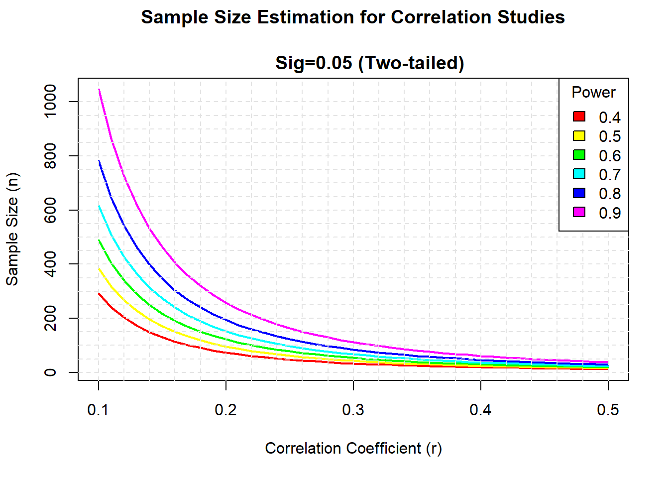
More examples at
Sample size in ANOVA (oneway)
(See theory at: )
(See examples at: )
library(pwr)For a one-way ANOVA comparing 5 groups, calculate the sample size needed in each group to obtain a power of 0.80, when the effect size is moderate (0.25) and a significance level of 0.05 is employed.
pwr.anova.test(k=5,f=.25,sig.level=.05,power=.8)##
## Balanced one-way analysis of variance power calculation
##
## k = 5
## n = 39.1534
## f = 0.25
## sig.level = 0.05
## power = 0.8
##
## NOTE: n is number in each groupSample size in ANOVA 2 FACTORS
(De http://www.evolutionarystatistics.org/document.pdf) Power Analysis by Simulation Frequently, the complexity of our experimental designs means that we must go far beyond what can be accomplished with standard software, such as the built-in power functions and the pwr package. Fortunately, R can be easily programmed to produce power analyses for any experimental design. The general approach is: 1. Simulate data under the null hypothesis (for checking Type I error probabilities) and also for different effect sizes, to estimate power. 2. Fit the model to the simulated data. 3. Record whether the analysis of the simulated data set was significant, using the usual tests. 4. Store the significance level in a vector. 5. Repeat from step 1. a large number of times. 6. Tabulate how many simulations produced a significant result, and hence calculate power. Here is an example: Suppose we wish to conduct a study with two fixed factor, leading us to a 2-way analysis of variance (ANOVA), with two levels for each factor. We could simulate data under the null hypothesis (no difference between means) using the following code:
## First set up the design
reps <- 1000
design <- expand.grid(A=c("a", "b"), B=c("c","d"), reps=1:10)
pvals <- vector("numeric", length=reps)
## simulate data under the null hypothesis.
for (i in 1:reps) {
design$response <- rnorm(40) # random data with zero mean
## fit the model
fit <- aov(response~A*B, data=design)
## record the p-value for the interaction term.
## You could record other values.
## Save the p value
pvals[i] <- summary(fit)[[1]][[5]][3]
}
Type1 <- length(which(pvals < 0.05))/reps
print(Type1)
## [1] 0.057It appears that the Type I error rate is acceptable for the 2-factor ANOVA interaction term. Now to calculate some power statistics. We will calculate power for a difference between means of 2 units, for sample sizes 5, 10, 20.
ssize <- c(5, 10, 20)
pvals <- matrix(NA, nrow=reps, ncol=3)
## First set up the design
for (j in 1:3) {
reps <- 1000
design <- expand.grid(reps=1:ssize[j], A=c("a", "b"), B=c("c","d"))
## simulate data under the null hypothesis.
for (i in 1:reps) {
design$response <- c(rnorm(3*ssize[j]), rnorm(ssize[j], mean=2))
## fit the model
fit <- aov(response~A*B, data=design)
## record the p-value for the interaction term.
## You could record other values.
## Save the p value
pvals[i,j] <- summary(fit)[[1]][[5]][3]
}
}
Power <- apply(pvals, 2, function (x) length(which(x < 0.05))/reps)
names(Power) <- as.character(ssize)
print(Power)
## 5 10 20
## 0.555 0.848 0.999We see that the power is too low for a sample size of 5, but it increases to an acceptable level for 10 replicates per treatment.
BIBLIOGRAPHY
MONLEON T, RODRIGUEZ C. Probabilitat i estad?stica per a ci?ncies I. PPU. BARCELONA. 2015.
ALCA?IZ M., GUILLEM M., PONS E. i RUFINO H. Problemes d’estad?stica descriptiva. Publicacions i Edicions UB. ISBN 978-84-475-3816-4.
BESAL? M i ROVIRA C. 2013. Probabilitats i estad?stica. Publicacions i Edicions UB. ISBN: 978-84-475-3653-5.
BONFILL, X.; BARNADAS, A.; CARRE?O, A.; ROSER, M.; MONLE?N, T.; MORAL, I.; HERN?NDEZ-BOLUDA, J. C.; P?REZ, P.; LLOMBART, A. (Coordinaci? Roset, M. / Monle?n, T.) (2004). Metodolog?a de investigaci?n y estad?stica en oncolog?a y hematolog?a. EDIMAC.
CUADRAS, C. M. [et al.]. Fundamentos de estad?stica. Aplicaci?n a las ciencias humanas. Barcelona : EUB, 1996.
CUADRAS, C. M. Problemas de probabilidades y estad?stica. Vol. 1: Probabilidades. ed. corregida i ampliada Barcelona : EUB, 1999-2000.
CUADRAS, C. M. Problemas de probabilidades y estad?stica. Vol. 2: Inferencia estad?stica. ed. corregida i ampliada. Barcelona : EUB, 1999-2000.
DAVIS, J. C. Statistics and data analysis in geology. 3a ed. New York [etc.] : Wiley, cop. 2002. JEKHOWSKY, B. DE ?l?ments de statistique ? l’usage des g?ologues. Par?s : Technip, 1977.
JULI? DE FERRAN O., M?RQUEZ-CARRERAS D., ROVIRA ESCOFET C. i SARR? ROVIRA M. 2003. Probabilitats: problemes i m?s problemes. Publicacions i Edicions UB. ISBN 978-84-475-2906-3.
JULI? O. i M?RQUEZ-CARRERAS D. Un primer curs d’estad?stica. 2011. Publicacions i Edicions UB. ISBN: 978-84-475-3483-8.
MILLER, R. L.; KAHN, H. N. Statistical analysis in the geological sciences. New York : Wiley, 1962. S?NCHEZ ALGARRA, P. (coord.) M?todos estad?sticos aplicados. Barcelona. Publicacions i Edicions de la Universitat de Barcelona, DL 2006.
MONLEON, A.; BARNADAS, A.; ROSET, M.; HERN?NDEZ-BOLUDA, J. C.; P?REZ, P.; LOMBART, A. (coordinaci? Monle?n, T.) (2005). Metodolog?a de investigaci?n y estad?stica en oncolog?a y hematolog?a (Casos Pr?cticos). EDIMAC.
Monleon, T. (2009). Manual de introduccion a la simulacion de ensayos clinicos. (pp. 1 - 182). Publicacions i Edicions UB. ISBN: 97978-84-475-3181.
MONLEON, T. (2010). El tratamiento numerico de la realidad. Reflexiones sobre la importancia actual de la estadistica en la Sociedad de la Informacion. Arbor, 186(743), 489-497. ISSN: 0210-1963.
MONLEON, T.; BARNADAS, A.; ROSET, M. (2008). ?Dise?os secuenciales y an?lisis intermedio en la investigaci?n cl?nica: tama?o versus dificultad?. Medicina Clinica, 11(132), 437-442. http://www.clinicasdenorteamerica.com/clinicas/ctl_servlet?_f=3&pident=13134609 ISSN: 0025-7753
MONLEON, T.; COLLADO, M. (2008). Tecnicas de control estadistico de procesos y software. Calidad industrial del trigo y la harina?. Alimentaci?n, Equipos y Tecnolog?a, 238, 50-54. ISSN: 0212-1689
SANCHEZ ALGARRA, P. (coord.) M?todos estad?sticos aplicados. Barcelona. Publicacions i Edicions de la Universitat de Barcelona, DL 2006.
STIGLER, S. M. (1990). The History of Statistics: The Measurement of Uncertainty before 1900. Belknap Press/Harvard University Press. ISBN 0-674-40341-X.